One parameter of interest in survival analysis is the median residual at time x.
Recall the definition of survival function, the probability of a subject experiencing the events beyond time x , defined as $S(x)=Pr (X >x) $, X is a continuous random variable.
The pth quantile is found by solving \(S(x_p)=1-p\). For example, the median lifetime is the 50th percentile \(x_{0.5}\), the 75 percentile lifetime is the 70th percentile \(x_{0.75}\). These are obtained by solving the following: \(S(x_{0.5})=1-0.5=0.5\), \(S(x_{0.75})=1-0.75=0.25\).
In Kaplan Meier estimate, we find the smallest time \(x_p\) for which the product limit estimator is less than or equal to 1-p. That is \[ \hat{X_p}= inf [ t: \hat{S} (t) \le 1-p ] \]
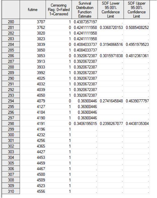
The LIFETEST procedure in SAS provides the survival time estimate in the table below:
proc lifetest data=pbc outsurv=km_sur2
plots=survival( cl test atrisk (maxlen=13) nocensor) maxtime=4000 notable ;
time futime*status(0,1);
strata drug;
run;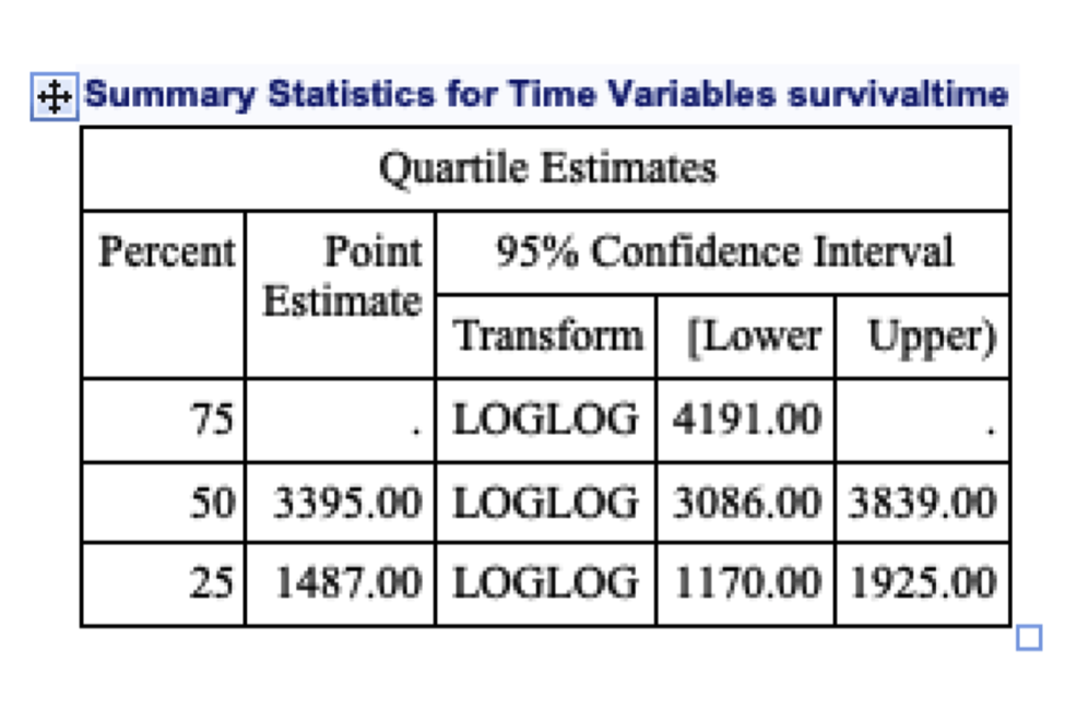
The missing 75th percentile survival time is because the maximum survival probability that could be determined is 0.34 in this study data (see the below figure).
In Kaplan Meier method, the estimator is appropriate only when the largest observation corresponds to a event. A Kaplan-Meier estimator is well defined for all event time points less than the largest observation time, and is NOT defined in other times. If the largest study time is a event , the survival curve is zero beyond this point. If the largest time point is censored the value of \(S(t)\) beyond this point, the Kaplan Meier survival estimate is undetermined. These are the reasons that you may see the survival output data had missing estimators in those non-event times.